Introduction
In order for researchers to perform effectively with the assistance of the advisors, the SPSS Assignment assistance for students is effectively helping in achieving educational success. In order to help the participants improve their performance in the near future, the consultants aim to mentor and support them as they learn new knowledge and learning skills. The article’s main objective is to analyze the benefits of student assignments and SPSS assignment assistance in the academic sector. It is feasible to investigate the advantages of such solutions in the career by critically studying the SPSS assignments to help students’ actions. Students are looking for knowledgeable SPSS assignment help for students and composing help groups to have continuous assistance from them so that they can effectively complete their study and thesis papers within the given timeframe.
Statistical Need homework assistance for students
Achieve greater results
Students might improve their grades on their assignments by using SPSS homework assistance. The pupils can’t do useful assignments, which is the cause. This enables them to give them high-caliber work. They can thus achieve good grades in their work.
Awareness of the topic in detail
Students may fully comprehend the SPSS material with the aid of SPSS assignment assistance. It is rare for students to pay attention in class long enough to grasp the concepts of SPSS. They gain greater knowledge about SPSS thanks to this assistance. Since the specialists are providing this assistance, they are prepared to assist students in learning the fundamentals of SPSS.
Improved Preparation
This assistance is highly helpful for students to better prepare for their examinations. They can easily receive a high grade as a result of it. To get their questions answered, students can consult professionals. Thus, it aids in their ability to plan ahead more effectively.
Effective Work
Students can obtain high-caliber work from specialists with the use of this assistance. There are several organizations that offer SPSS homework assistance. All of these professionals give the pupils high-quality work.
Saving time
The most valuable resource in the world at the moment now is time. Additionally, students desire to save time. Because it saves them valuable time, SPSS assignment assistance is essential for them.
Conclusion
The SPSS assignment help, which is beneficial to all students, is helpful in supporting higher assistance to the students by providing a variety of data analysis techniques and methodologies, allowing participants to select the most appropriate approach for doing strategic research. Additionally, the researchers have the chance to expand their knowledge and skills in order to work more effectively and achieve their goals, thanks to the SPSS assignment assistance for students. Reliability in getting a degree as well as improved practical skills and knowledge in market data collection and data analysis are other benefits that help researchers perform better and comprehend the dissertation and thesis writing process. Thus, using the SPSS assignment assistance and writing services, students may manage their tension, lessen their anxiety about participating in research, and enhance their own ability to do market research as well as data analysis. Students may progress in their careers and succeed professionally with the SPSS assignment to help them through communication and understanding.
Our SPSS Experts have prepared sample assignment solution to demonstrate the quality of our work. All the solutions have been prepared by following a simplistic approach and include step by step explanations. These solutions reflect the in-depth expertise and experience of our online SPSS assignment experts.
Paired t-test and One-Way Repeated-Measures ANOVA Stretch
QUESTION: SPSS Assignment
Open the SPSS data file in your In-Class Exploration folder. It contains data from a made-up study about revelers at the Glastonbury Music Festival in England. The Glastonbury Music Festival runs across 3 days, and you – in your researcher capacity – have noticed a certain “ripeness” amongst the concert-goers. You wonder whether hygiene is related to the type of music the concert-goers prefer. You rate concert-goers’ smell on a scale of 0 (sewer) to 4 (freshly baked bread) and you ask them to report their musical affiliation. From their responses, you categorize them into four groups (Indie Kid, Metaller, Crusty, and No Musical Affiliation).
We’ve already examined how hygiene differs as a function of musical affiliation only on Day 1 of the festival. Now, we will examine change over time, or a repeated measurement. So, the null hypothesis is: Time does not affect hygiene in the population.
What is the IV? How many levels does it have?
What’s the DV?
What do higher scores on the DV mean?
The appropriate test to analyze these data would be a…
This procedure mimics what you will need to do in Independent Practice 6. (DISCLAIMER: In a real study you wouldn’t perform a t-test and then follow it up with an ANOVA, but I’m trying to get the biggest bang for our buck with a single dataset while ensuring that you have practice conducting each type of test.) Follow the steps listed below, then check your output against the output provided. Answer the questions that are interspersed within this guide.
Step-by-step instructions:
- Click on “Variable View” or “Data View” tab (doesn’t matter!).
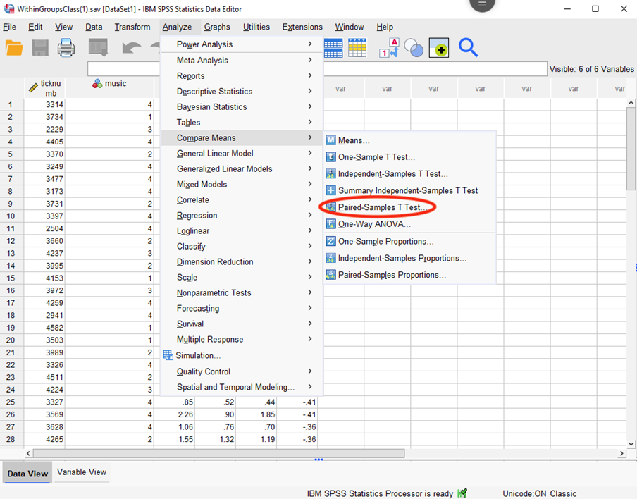
- Let’s compare Day 1 and Day 2. The null hypothesis is: The difference in hygiene between Day 1 and Day 2 is zero ITP. Select Analyze, Compare Means, Paired samples t-test.
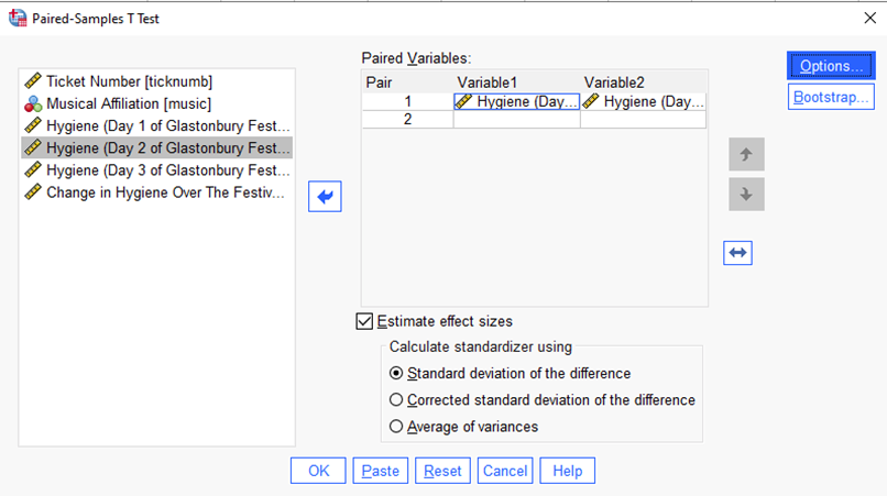
Drag the two levels that you want to compare (Hygiene on Day 1 of the Festival, Hygiene on Day 2 of the Festival) into the Paired Variables box. Hygiene for Day 1 should be placed under Variable 1; Hygiene for Day 2 should be placed under Variable 2. This labeling is unfortunate – remember that you do not have two VARIABLES here. You have two LEVELS or CONDITIONS of your IV. Ensure that “Estimate Effect Size” is checked and “Standard Deviation of the Difference” is selected. It should look like this:
- Click OK. Your output should look like this:
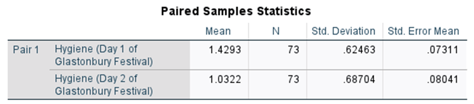
The first table provides descriptive statistics (mean, n, standard deviation, and standard error of the mean). If you were to report descriptive statistics in APA style for Day 1, it would look like: (M = 1.43, SD = 0.62).
How would you report descriptive statistics for Day 2?
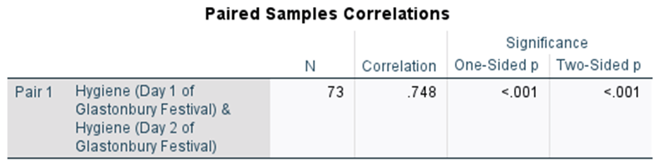
The second table tells you whether the scores for each level of your IV are correlated using a Pearson r correlation.
We’ve worked with Pearson r correlations before. How would you interpret this correlation?
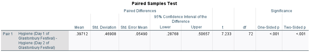
The Paired Sample Test table first gives you the difference between the means (Mean for Day 1 – Mean for Day 2). The t-test evaluates whether the difference between the means is significantly different from zero (no difference). The 95% confidence interval of the difference is interesting to look at. If the confidence interval does not include 0, your difference between the means is likely to be different from zero (i.e., there is a real difference between the means) ITP. Next we have our t value (7.23), df (72), and Sig. (2-tailed) or p value (<.001). So, p < .001 and we can reject the null hypothesis and state: Hygiene significantly declines between Days 1 and 2 of the Festival.
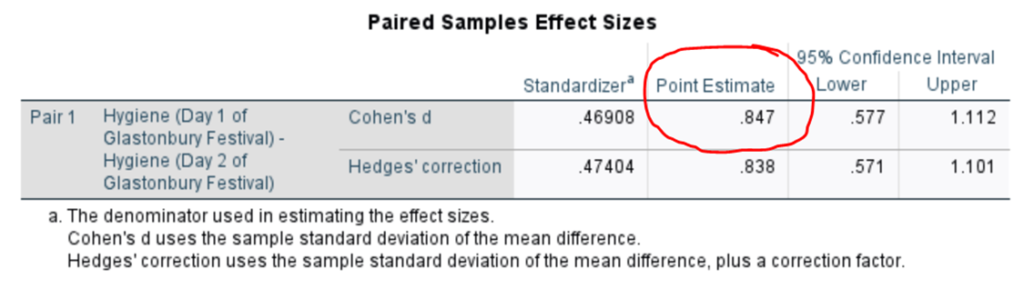
On to effect size. Again, we’ll use Cohen’s d, which tells you how many standard deviations the difference between the means is from zero. The farther away the mean difference from zero, the stronger the effect/relationship.
So, Cohen’s d is 0.85, which indicates that the means of the groups are half a standard deviation apart. That’s a medium-sized, or moderate effect. Consult the table below for interpreting/labeling Cohen’s d effect size:
- ±.2 indicates a small effect
- ±.5 is a moderate effect
- ±.8 is a large effect
Note that Cohen’s d can be positive or negative. Further, the 95% Confidence Intervals are the upper and lower bound of this effect size. In other words, if I ran this study 100 times, I would find Cohen’s d values within the bounds of 0.41 and 0.79 95 out of 100 times. So, I could find a slightly moderate effect or a large one.
Now that we have effect size, we can write the t expression in APA style. It starts with “t” followed by degrees of freedom in parentheses, then the t value, the p value, and Cohen’s d and the 95% CI around the mean difference:
t(72) = 7.23, p < .001, d = 0.85, 95% CI [ 0.29, 0.51]
Optional challenge: Examine the difference in hygiene between Day 2 and Day 3. Write the findings in APA style.
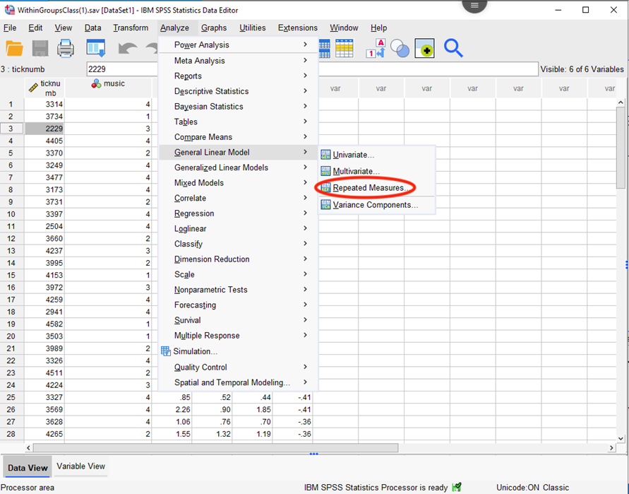
- Now we move to the one-way Repeated-Measures ANOVA. The null hypothesis states that the differences in hygiene across all days of the festival are equal to Zero ITP. Select Analyze, General Linear Model, Repeated Measures.
In the resulting dialogue box, you need to label your factor. We have 1 IV (Days) with three 3 levels (Day 1, Day 2, and Day 3). Type “Days” in the Within-Subject Factor Name box. Type “3” in the Number of Levels box. Click Add. It should look like this:

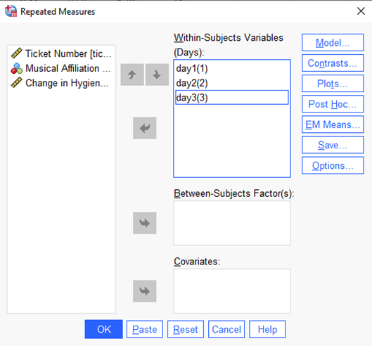
Click Define to advance to the next screen. Next, you need to assign the three levels of your IV in the Within-Subjects Variables (Days) box. Drag the three Hygiene levels into the three slots awaiting them in the Within-Subjects Variables box. Remember, you do NOT have 3 IVs; you have 3 levels of 1 IV. Click Continue and you should see:
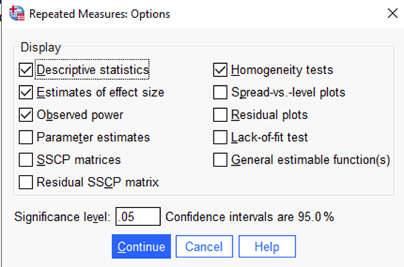
Click Options. Select Descriptive Statistics, Estimates of Effect Size, Observed Power, and Homogeneity Tests. (In truth, you don’t need homogeneity tests because you don’t have any between- participant IVs. It doesn’t hurt anything to check it and I’d rather you get in the habit anyway!).
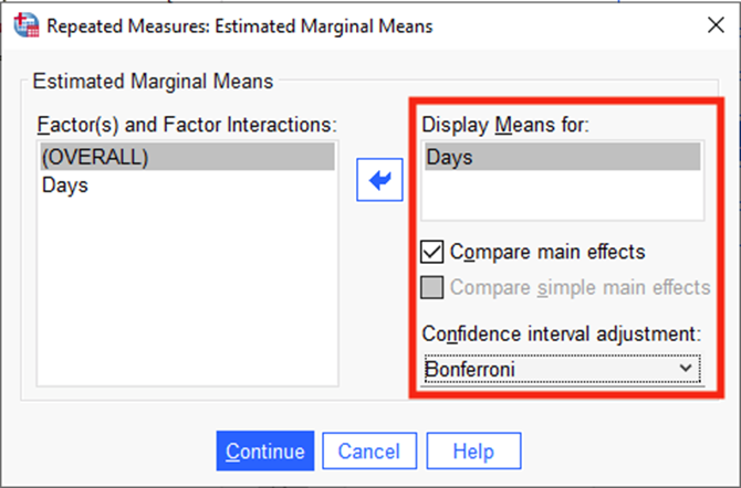
Click Continue. Click EM Means (which remember stands for Estimated Marginal Means). Drag Days over to Display Means for. Click the Compare main effects box. Select Bonferroni from the drop-down menu for Confidence interval adjustment. This will give us Pairwise Comparisons across the different days (like post-hoc tests for independent groups).
- Click Continue. Here comes your output.
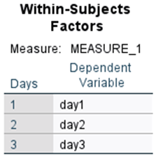
The first table (Within-subjects factors) just tells you what your variables and levels are. SPSS labels each level of your IV as a dependent variable because it conducts a MANOVA on the data as well as a Repeated-Measures ANOVA. You’ll learn why SPSS does this as we progress through the output….
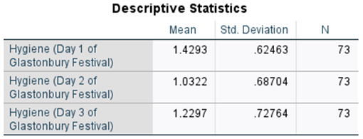
Next is the Descriptive Statistics table. You see means, standard deviations, and n for each day of the festival. Why should N always be the same number in this table?
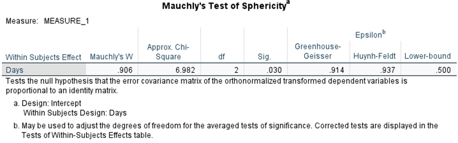
We’re going to skipover the Multivariate Tests table for the moment and head down to Mauchly’s Test of Sphericity. Mauchly’s test is essentially a test of homogeneity of variance across the distributions of the difference scores. Here, we want those variances of the differences to be equal to each other. In other words, we want to fail to reject the null hypothesis that the variances of the difference scores across conditions are equal to each other. We do NOT want to reject that hypothesis! If we reject it, that means we have violated the assumption of sphericity (that the variances between the distributions of the difference scores are equal). So, we look at the p (Sig.) value. If the value is greater than .05, we have NOT violated the assumption of sphericity. If the value is .05 or less, we have violated the assumption of sphericity.
Ruh-Roh… p = .030. We’ve violated sphericity. What do we do? Go up one table in the output and read the Multivariate Tests table. You interpret this table just like you did when learning the MANOVA (because it is a MANOVA). Now you know why that first table in the output labeled Days of the Festival as three separate DVs. When we violate sphericity, we need to be more conservative about deciding whether to reject he null hypothesis. Running the analysis as a MANOVA offers that added bit of security.
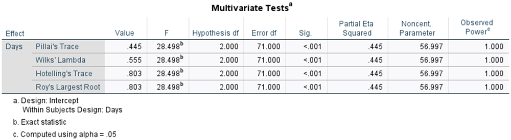
So, from the MANOVA output, we reject the null hypothesis, because p < .001. Thus, at least two of the means of the difference scores across the three days of the festival are significantly different from each other. How would you write the findings in APA style? Fill in the blanks:
Wilks’ L = ____, F(___, ____) = _______, p _______, hp2 = _______.
What would happen if you did not violate sphericity? You would evaluate the Tests of Within-Subjects Effects table:
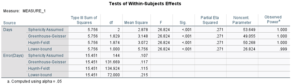
You would read the row that states “Sphericity Assumed”. The p value is less than .05, so we reject the null hypothesis. How would you write the findings in APA style? Fill in the blanks:
F(___, ____) = _______, p _______, hp2 = _______.
All that’s left to do is evaluate which of the difference scores significantly differ from zero (so many “differs”!). The omnibus Repeated-Measures ANOVA or MANOVA just tells us that there’s a difference somewhere – neither tells us where that difference resides.
Ignore the Tests of Within-Subjects Contrasts and Tests of Between-Subjects Effects tables. Go to the Pairwise Comparisons table:
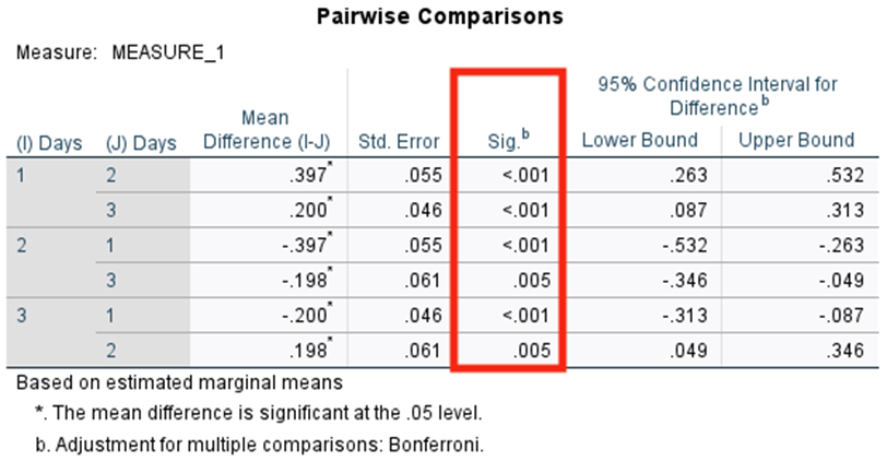
We look at the Sig. column. If any of the values are .05 or less, we know that the difference between the two means that SPSS is comparing is different from zero (i.e., there’s a significant difference between the means). From these p values, it looks as if all means are different from each other!
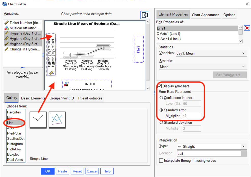
- Now we have to visually represent the results in a bar graph. Select Graphs and Chart Builder (if you get the message about making sure your variables are labeled correctly, hit OK). The default is set to Bar graphs and we’re going to choose a Simple Line graph (the first from the top left) and drag it to the Canvas. Highlight all three levels of the IV (Hygiene Day 1, Hygiene Day 2, Hygiene Day 3) in the Variables box using the control or the shift key. It is very important that all three levels are highlighted. Drag the levels to the Y axis. Hit OK to the dialogue box that appears about creating an INDEX variable (you saw this doing that MANOVA graph.
Click on Display error bars and select Standard error with a Multiplier of 1 (the default is 2 multiplier, or 2 standard errors around the mean). Why not 95% CI? In SPSS, 95% CI’s are calculated on the basis of a between-participant comparison. There is a way to adjust for a within-participant comparison, but I’m not going there with you! J
You should see something like:
Click OK.
You’ve got your figure, but you need to clean up the format. Double click the figure to open the Chart Editor where you can change elements of the figure. We need to:
Remove the title at the top of the figure (you’ll type a different one in your write-up!)
Remove the notes about error bars at the bottom of the graph.
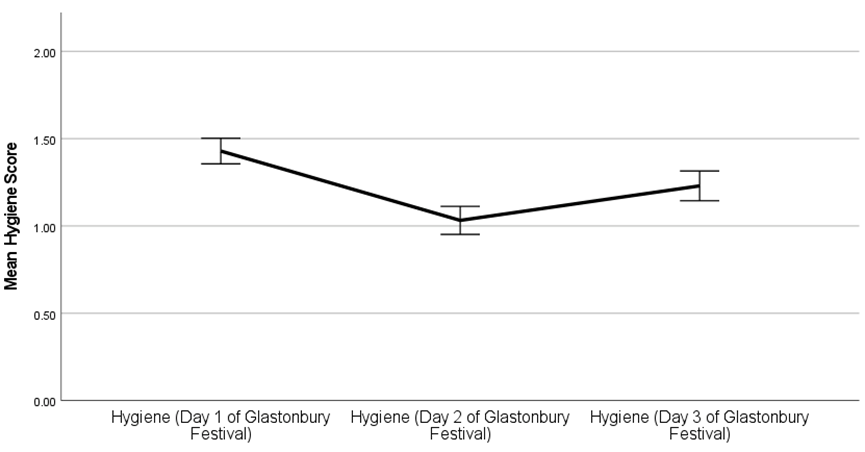
When you are finished editing, it should look like this:
And you’re done! Whew! Now’s your chance to write this up. Please be aware that this template COMBINES the paired t-test and the one-way repeated-measures ANOVA. You would not do it this way in practice! (You would choose the appropriate test and use only that one.) But this is how you need to proceed for Independent Practice 6.
SOLUTION:
Premilnary Analysis
I conducted a paired sample t-test to compare whether the hygiene level at festival day 1 differs from that of day 2. Hygiene level at day 1 differs significantly (M=1.43, SD=0.62) to that of day 2(M=1.03, SD=0.69), t(72) = 7.23, p< .001, d = 0.85, 95% CI [0.29, 0.51].This difference is quite strong and would likely be strong in the population (95% CI [0.29, 0.51]). As indicated in Figure 1, the error bars do not overlap.
I conducted one-way repeated-measures ANOVA with days (day 1, day 2, day 3) as the independent variable and Hygiene level as the dependent variable. Hygiene level significantly differs over the three days, F(2,144) = 26.824, p< .001, partial η2 = .27. This relationship is strong, with days accounting for 27% of the variation in hygiene level.
Pairwise comparisons using a Bonferroni correction revealed that hygiene level decreased significantly different from day 1 (M = 1.43, SD = 0.62) to day 2 (M = 1.03, SD = 0.69), p <.001, and at day 3 (M = 1.23, SD = 0.73), p< .001. Further, level of hygiene increase significantly from day 2(M = 1.03, SD = 0.69) compared to day 3 (M = 1.23, SD = 0.73), p< .001. Lastly, as illustrated in Figure 1, the error bars across all conditions do not overlap.
Figure 1
Level of hygiene as a function of days (day 1, day 2, day 3)